Capital Assets Pricing Model

import numpy as np
import matplotlib.pyplot as plt
import pandas as pd
import datetime as dt
import yfinance as yf

plt.style.use("ggplot")
import statsmodels.api as sm

Unsystematic risks can be diversified. Systematic risks can’t be diversified, \(\text{CAPM}\) measures this risk with \(\beta\).

\[ \begin{aligned} E(R_i)= & R_f+\beta_i[E(R_m)-R_f] \end{aligned} \]

\[ \begin{array} E\left(R_i\right) & =\text { capital asset expected return, e.g. a single stock or a portfolio } \\ R_f & =\text { risk-free return, e.g. 10y treasury bond} \\ \beta_i & =\text { sensitivity } \\ E\left(R_m\right) & =\text { expected return of the market, e.g. S&P500 } \end{array} \]

\(\beta_i\) can be calculated by OLS formula, i.e. \[ \beta= \frac{\text{Cov}(R_i, R_m)}{\text{Var}(R_m)} \] it tells how risky your portfolio is relative to the market, it only measures the systematic risk.

The portfolio \(\beta\) will be a weighted \(\beta\) \[ \beta = \sum_{i=1}^n w_i\beta_i \]

The model can be rewritten as \[\begin{aligned} E(R_i)-R_f= \alpha_i+\beta_i[E(R_m)-R_f] \end{aligned}\]

to explicitly estimate \(\alpha\) as a constant. It characterizes the excess rate of return that

\[ \alpha_i= E(R_i)-\{R_f+\beta_i[E(R_m)-R_f]\} \] Usually the classic CAPM assumes \(\alpha=0\)

In short, \(\beta\) measures systematic risks, \(\alpha\) measure excess returns.

Implementation of CAPM

class CAPM:
    def __init__(self, stocks, start_date, end_date):
        self.stocks = stocks
        self.start_date = start_date
        self.end_date = end_date

    def download_data(self):
        stock_data = {}
        for stock in self.stocks:
            ticker = yf.Ticker(stock)
            stock_data[stock] = ticker.history(
                start=self.start_date, end=self.end_date
            )["Close"]
        return pd.DataFrame(stock_data)

    def resample_month(self):
        # montly return gives a better normally distributed results
        stock_data = (
            self.download_data()
        )  # without this, 'stock_data' will be called before assignment
        stock_data = stock_data.resample("M").last()
        self.data = pd.DataFrame(
            {
                "s_adjclose": stock_data[self.stocks[0]],
                "m_adjclose": stock_data[self.stocks[1]],
            }
        )
        self.data[["s_logreturn", "m_logreturn"]] = np.log(self.data) - np.log(
            self.data.shift()
        )
        self.data = self.data.dropna()
        return self.data

    def calculate_beta(self):
        cov_matrix = np.cov(self.data["s_logreturn"], self.data["m_logreturn"])
        self.beta = cov_matrix[0, 1] / np.var(self.data["m_logreturn"])
        print(self.beta)
        return self.beta

    def lin_reg(self):
        R_F = 0.05
        month_in_year = 12

        X = self.data["m_logreturn"] - R_F
        Y = self.data["s_logreturn"] - R_F
        X = sm.add_constant(X)  # adding a constant
        self.results = sm.OLS(Y, X).fit()
        alpha, beta = self.results.params[0], self.results.params[1]
        expected_return = R_F + beta * (
            self.data["m_logreturn"].mean() * month_in_year - R_F
        )
        self.plot_regression()
        print("alpha: {}".format(alpha))
        print("beta: {}".format(beta))
        return alpha, beta, expected_return

    def plot_regression(self):
        fig, ax = plt.subplots(figsize=(6, 6))
        ax.scatter(
            self.data["m_logreturn"], self.data["s_logreturn"], c="CornflowerBlue"
        )
        ax.plot(self.data["m_logreturn"], self.results.fittedvalues)
        ax.set_title("Capital Assets Pricing Model: {}".format(stocks[0]))
        ax.set_ylabel("Expected Stock Return")
        ax.set_xlabel("Expected Market Return")
        plt.show()


if __name__ == "__main__":
    stocks = ["LULU", "^GSPC"]
    capm = CAPM(stocks, start_date="2010-01-01", end_date=dt.datetime.today())
    data = capm.download_data()
    data_month = capm.resample_month()
    beta_calculated = capm.calculate_beta()
    alpha, beta, exp_ret = capm.lin_reg()

1.2162665097364047

/tmp/ipykernel_3463/4094164405.py:21: FutureWarning:

'M' is deprecated and will be removed in a future version, please use 'ME' instead.

/tmp/ipykernel_3463/4094164405.py:48: FutureWarning:

Series.__getitem__ treating keys as positions is deprecated. In a future version, integer keys will always be treated as labels (consistent with DataFrame behavior). To access a value by position, use `ser.iloc[pos]`

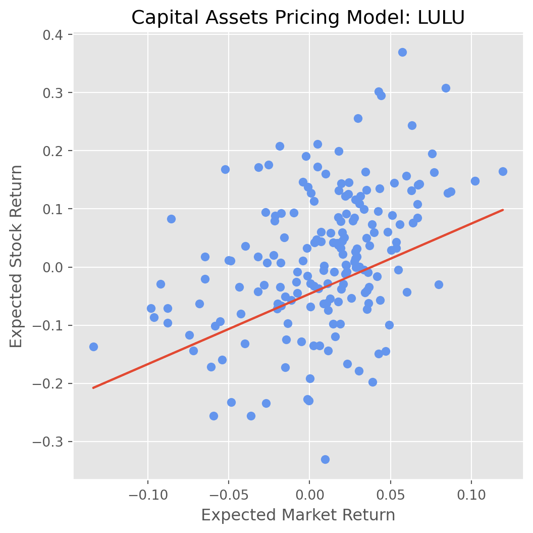
alpha: 0.014293598162767422
beta: 1.2096920961702622